
Time series forecasting algorithms still stand as one of the essential factors in deciding how the market will perform in the future, in regards to time. Whether time series forecasting algorithms are about determining price trends of stocks, forecasting, or sales, understanding the pattern and statistics involving time is crucial to the underlying cause in any organization.

Definition of Time Series Analysis
Time-series data is simply a set of ordered data points with respect to time. The analysis is comprised of different algorithms or methods used to extract certain statistical information and characteristics of data, in order to predict the future values based on stored past time-series data.
“Prediction is truly very difficult, especially if it’s about the unknown future”
– Nils Bohr, Nobel laureate in Physics
It is essential to validate a forecasted model. It’s often easy to find a model that fits the past data well. Still, quite another matter to find a model that correctly identifies those patterns in the past information that will continue to hold in the future.
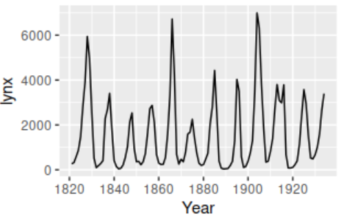
Moreover, time-series data is commonly plotted on a line graph. This is because the individual data points are spaced equally with time, hence time becomes an independent variable with respect to the data being investigated. It is presented in that way so that the correlation (if exist) could be visualized easily.
Where is Time-Series analysis used?
Time Series helps in analyzing the past data, which then becomes an essential factor in forecasting the future. Time series forecasting is crucial in most organizations in determining the actions and decisions that will be taken.
Organizations perform that by collecting large amounts of past data and compare them to the current trend, thus making holistic decisions. Below are 2 of the use cases of Time Series forecasting, where it is extensively applied.
1. Stock Market Analysis
Stocks prices are actually discrete-time models where the data points (e.g price) are independent of the time. Using Time Series forecasting and Algorithms, some of the important components such as Trend and Seasonality can be derived to allow the investors to predict the movement of the price.
2. Budgetary Analysis
For an organization, maintaining a steady income of cash flow is important as it allows the stakeholders to provide a reliable forecast of its revenues and expenditures in that financial year. That is why budgeting is important. It allows businesses to plan ahead the budget for the next year, based on the current year’s allocation and expenses.

Popular Algorithms in the Industry
Below are the 5 most commonly used algorithms in the industry, let it be in banking, finance, engineering, etc. All of the algorithms below tend to perform some form of trivial analysis of the data that were given to figure out some of the important characteristics for forecasting purposes.
Autoregressive (AR)
Autoregressive model learns the behavioral pattern of the past data in order to do time series forecasting of future trends.
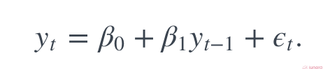
In the regression model, the response variable in the previous time period has become the new predictor, and the errors have been assumed about errors in any simple linear regression model. It is simple to understand this.
Notice that in the equation, for a prediction of time t, it relies on t-1 and so on all the way till t-n. This is called lagged prediction since it relies on data points that are in the previous period of time.
The autoregressive model is a stochastic process, which involves some form of the randomness of data with time. The randomness (or fluctuations) signifies that you might be able to predict future trends in high accuracy with the past data, but just not close enough to be 100% accurate. An example use case of the AR algorithm and model is to predict the daily temperature in a particular area over X years.
Moving Average (MA)
Unlike the AR model where it uses past data to predict trends, The Moving Average algorithm uses past forecasted errors (or noise) in a regression-like model to elaborate an averaged trend across the data.
Moving average can be defined as the weighted sum of the current random errors and the past errors as shown in the equation below:
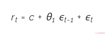
- c refers to some white noise with zero mean and small variance
- θ1 refers to the coefficient of the first data point
- ϵt-1 and ϵt refer to the past and current period respectively
Something to note is that Moving Average does not use past data points to forecast the future values, unlike Autoregression.
Autoregressive Moving Average (ARMA)
The ARMA algorithm is simply the combination of the above Moving Average and Autoregression. Autoregressive extracts the momentum and pattern of the trend whereas Moving Average capture the white noise effects, and the addition of this creates ARMA.
The ARMA algorithm is usually modeled using the Box-Jenkins method where it detects the presence of stationary, seasonality and differencing to apply a line of best fit to the data points.
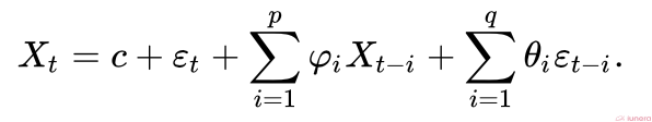
- p is the order of the Autoregressive model
- q is the order of the Moving Average model
In short, ARMA algorithm explains the relationship of a time series by using past values of itself (AR) with the combination of white noise (MA).
Autoregressive Integrated Moving Average (ARIMA)
ARIMA happens to be one of the most used algorithms in Time Series forecasting. While other models describe the trend and seasonality of the data points, ARIMA aims to explain the autocorrelation between the data points. Before getting into ARIMA algorithm, let’s discuss the basic concepts of ARIMA, stationary and differencing.
- A time series can be said to be stationary if the properties of the data do not change with time at that instant when it is observed. Time series with trends however are not stationary as the seasonality will affect the value at different times. In short, a stationary time series will have no predictable patterns in the long-term (constant variance)
- Differencing, however, is simply the result of the computation of the difference between consecutive stationary observations in the data points. It is usually applied to stabilize the average of a time series, therefore eliminating (or reducing) trend and seasonality.
An ARIMA algorithm-generated model then can be said as a differenced time series forecasting model to make it stationary.

- α represents some value of white noise
- p is the order of Autoregressive term (lagged predictions)
- q is the order of Moving Average (lagged errors)
Generally ARIMA is expressed in a format that looks like this:
ARIMA(p, d, q)
where d is the order of Differencing needed to make the time series stationary.
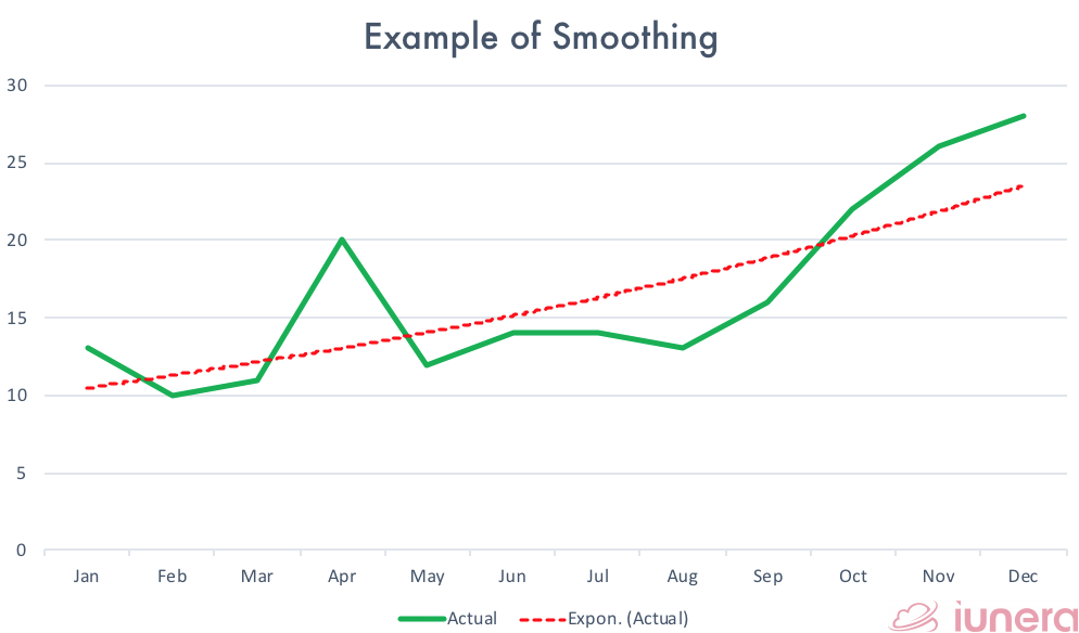
Exponential Smoothing (ES)
Exponential smoothing algorithm is used to produce a rather smooth time series forecasting trend whereby the older data values are exponentially decreased in weight, resulting in weighted averages. The degree of smoothing is adjusted (the width of the moving average), to optimize the model performance to a slowly varying mean.
This application of applying weights generates reliable forecasts quickly, which can be used to a wide range of time series forecasts and is a great advantage and of major importance to applications in the industry.
The simplest form of exponential smoothing can be expressed as below:

- α is the degree of smoothing ranging 0 < α < 1. In other words, how much importance is to be applied to that particular observation in that particular frame in time.
Depending on how the analysis is set, there is often an important trade-off between retaining the current observations or being constant. A high alpha value will allow the model to put more importance to the recent observation or changes — learns faster, whereas a smaller alpha is less susceptible to changes (ignores outliers and noise).
The exponential smoothing models are often called the “Holt-Winters” model. An early algorithm form of exponential smoothing forecast was initially proposed by R.G. Brown in 1956, whereby the equations were then further refined in 1957 by Charles C. Holt — a US engineer from MIT. The exponential smoothing models were again improved some years later by Peter Winters. This brings us finally to the model named above.
Exponential smoothing models are robust for any time series forecasting or analysis since it only requires a modest amount of computing power.
Conclusion
In summary, many different Time Series forecasting algorithms and analysis methods can be applied to extract the relevant information that is required.
Regardless of using Autoregressive algorithms to determine the trend patterns for forecasting or the ARIMA model to deduce the correlation pattern of the data, it all depends on the application use cases and the complexity. Since most time series forecasting analyses are trivial, choosing the easiest and simplest model is the best way to look at it.
Are you looking for ways to get the best out of your data?
If yes, then let us help you use your data.
Takeaway
2 use cases of time-series analysis
– Prediction of stock price movements.
– Forecasting revenues and expenditures for budget planning.
5 most common time-series forecasting algorithms
– Autoregressive (AR)
– Moving Average (MA)
– Autoregressive Moving Average (ARMA)
– Autoregressive Integrated Moving Average (ARIMA)
– Exponential Smoothing (ES)