Multidimensional Time Series Analysis VS OLAP

Multi-dimensional Time Series Analysis and OLAP methods are important when working with Time Series Data.

Often multi-dimensional Time Series Analysis (as the term is referred to) is a complete set of methods in applying machine learning to create forecasts or search for anomalies and patterns. Common multi-dimensional analysis operations get applied in Business Intelligence and Data Warehousing where they are often called Online AnaLytical Processing (OLAP) operations [1].

Knowing these multi-dimensional Time Series Analysis foundations is essential, because at least 80% of Data Science work is Big Data and Landscape preparation.

In this article, we focus on good old multi-dimensional Time Series Analysis foundations to prepare, investigate and aggregate the Time Series Data in a deterministic way. We also discuss and describe what the most important multi-dimensional Time Series Analysis and OLAP methods are and show examples of how the different operations are applied on a Time Series Data sets.

Why Data Warehouse OLAP VS Time Series Analysis?

Analytical multi-dimensional OLAP operations matter in the Big Data area, because Time Series Data can be processed and analyzed in the same way like data from a Data Warehouse. Multi-dimensional Time Series OLAP based Analysis is essentially applicable in Data Warehouses, which are classically filled with data out of operative enterprise systems.

Technologically, the multi-dimensional Time Series Analysis methods from Data Warehouses help to aggregate and generate subsets of Time Series Data in an efficient way.

These multi-dimensional analysis foundations from Data Warehouses are needed by Data Scientists to assess Time Series Data quality and to prepare the data then to apply the ultimately fancy Time Series Data.

Out of the pure volume, rare data deletion, other data sources and complexity, Big Data landscapes are realized with different technology stacks.

Data Scientist and Big Data Engineers combine classically multiple open source systems and leverages functionality in similar to a Data Warehouse in Big Data landscapes.

Time Series Databases often offer support for a subset of the complete analytical multi-dimensional operations which are available in Data Warehouses. Similarly, a Data Scientist can code and apply the operations by hand when investigating Time Series Data sets.

Hence, it helps to know the origin of the operations and how they work in order to apply them manually on Big Data or to leverage the right Time Series Database for this matter.

Why do we need multi-dimensional Time Series OLAP operations?

Just imagine the world of an executive:

Dozens of plants, hundreds of salesmen, thousands of employees and millions of sold products. How do you push the company in the right direction? Who are our star salesmen? Which are the most profitable products? Where and which products get sold the most?

These questions are asked by executives in order to steer a company and effective means to analyze the data in this way are needed. Therefore, one needs a simple way to compute different perspectives of the same data. Furthermore, one needs to view and get insights into specific subsets of the same data.

Data Scientists face the same issue as they need to determine which fraction of the Time Series Data they use to train AIs or to do descriptive Time Series Data analysis or investigations. Thus, they need ways to have data available in a pre-processed format to get the necessary perspectives easily when it is required, technology-wise or enterprise-wise.

Multi-dimensional Time Series Data foundations

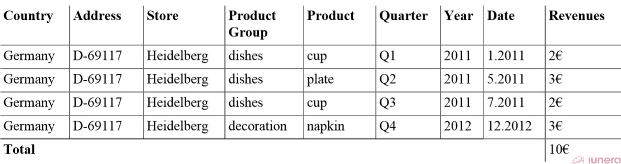
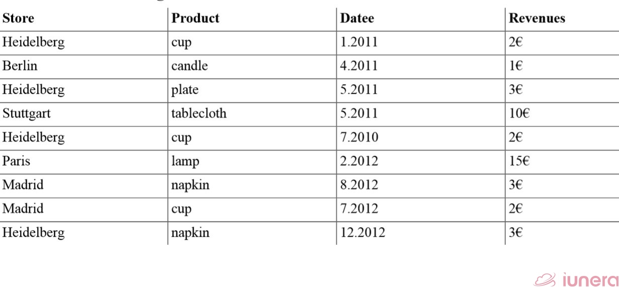
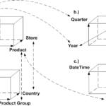
In the following, we use this sample dataset to help explain how multi-dimensional Time Series Data Analysis operations can be applied. We see that Date, Quarter and Year refer to Time Series Data and time intervals.

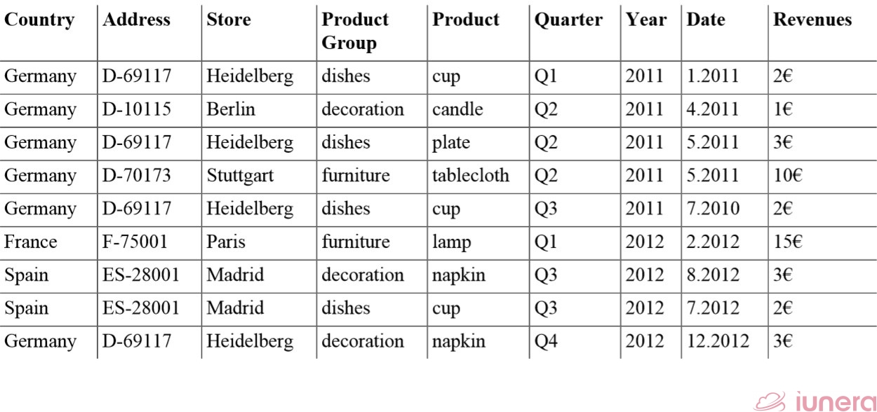
We show a schematic multidimensional arrangement of this data in the following graphic. The multidimensional arrangement is typically called cube or Hypercube in Data Warehousing.

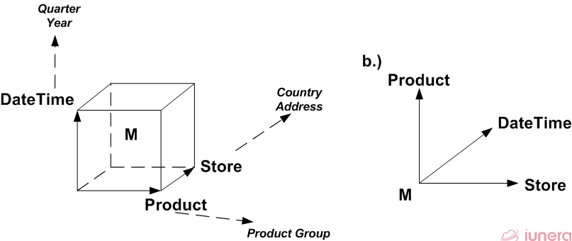
We see that the different columns are mapped onto dimensions and the revenues are represented by the measure (M) in the middle. Hence, the values of the columns link the indicator or revenues together.

In general, every dimension or attribute may be used as an element in a query to compute the revenues for the specified elements. For instance, such computation can be the revenues for a certain region within a certain time and for a certain product.

We also see that the dimensions can be seen as hierarchies such as the store and its located country. This way, one may compute totals and subtotals based on such hierarchies such as countries or the address.

How to Slice Time Series Data

Slicing is the operation of cutting a specific slice out of the data structure that is commonly applied when Time Series Data Analysis is done.

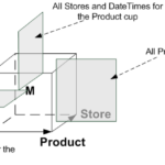
The data gets cut down to various dimensions, elements or attributes. We visualize different slices in the following image – there we see the slices for the various dimensions of the sample data.

We use a slice in the following. The slice of “All Stores and Dates for the Product cup” discriminates the dataset to the fixed value of a cup.

We see that just the stores in Madrid and Heidelberg are the remaining cup sellers. This way, decision-makers can easily view the total revenues for the cup product at hand and compare it with the totals. Then, they can use those totals to compare the different stores to the total revenues and see which store is the leading cup seller.

Similarly to the slice before, we present the slice of “All product and Dates for the Heidelberg Store” below. There we can see that the Heidelberg store sold three products for the total amount of 8€.

Out of this data, charts or other graphical visualization can be populated for a specific store. Such charts may give decision-makers insights into whether the revenues for a specific store increase over time. We show a simple visualization sample in the figure below.

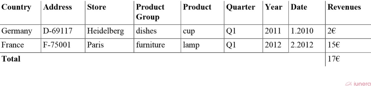
Lastly, we show the slice of “All Stores and products for the first Date Quarter”. We see that only Heidelberg and Paris sold products in Q1. Furthermore, the revenues compared to the total are much higher for Paris than for the Heidelberg store.

However, in general, such slices are the beginning of further Time Series analysis and the building of total sums and similar aggregations is a starting point to do advanced investigations.

Our example contained only limited cases that are easy to overview to demonstrate the general idea of how data can be sliced. In reality, we have to imagine thousands and millions of records that are hard to overview. Through slicing, the amount can be dramatically reduced.

Imagine not only to compute totals for Time Series Data but also subtotals and similar. For instance, subtotals may be computed for the specific stores, products and lead to new Time Series analysis insights.

Here, we focused on the generic approach to slice data, to reduce a result set and demonstrate advanced analysis capabilities later on. For us, it is important to note, that slicing fixes a dimension on a certain member (e.g. the specific store, location or interval) in order to reduce the original dataset.

Dice Time Series Data in a subcube

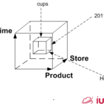
Similar to the slice operation discussed – is the Dice operation. The dice operation combines multiple slice operations at one time to create a subcube.

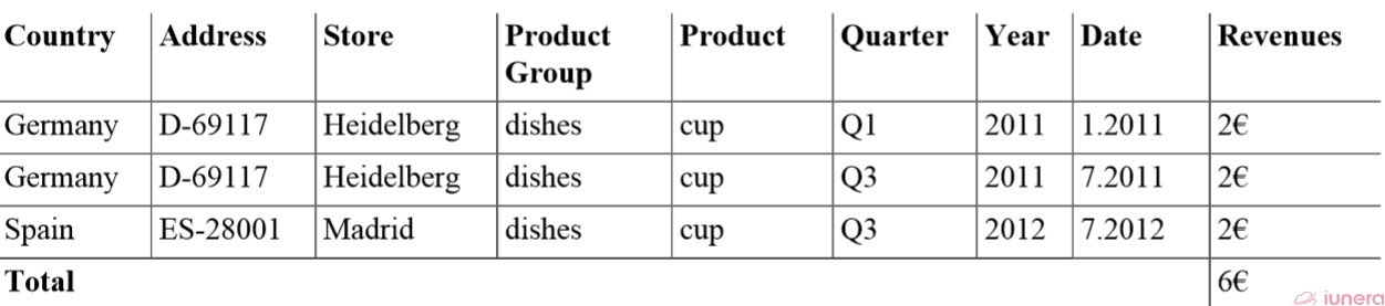
In the picture, we see how different dimensions are fixed to specific values and a subcube is extracted. For our demo data, we present the remaining subcube in the following table.

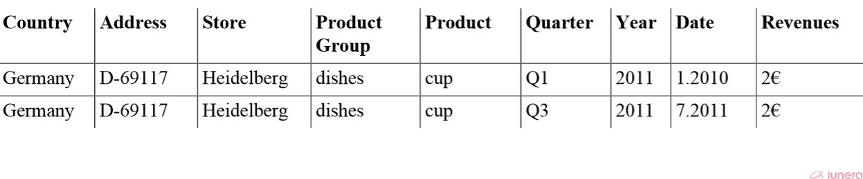
The table shows that two datasets remain. Furthermore, neither slicing nor dicing change the dimensionality of the Time Series Data. All dimensions that were existing before are still remaining in the result.

In general, such a Dice operation is often used to start analysis for a specific entity. Imagine a local executive who is responsible for the Heidelberg store and wants to do the future planning for the store in Heidelberg for 2012.

He needs to determine how many cups he needs now and how many he has needed in the past periods to go into negotiations with the cup vendor. In order to do so, he is interested in the historical data of the year 2011 for his specific store.

He is not interested in the data of the whole company and focuses on his store. So, all computations that he wants to do are based on the Heidelberg- 2011- cup -result. If he would look at the whole company data, it would be overwhelming and unimportant information for him.

Advanced Operations

Before, we discussed the basic Slice and Dice operation as Time Series Analysis methods. We saw that the data representation was uniform and the operations can be used to reduce the dataset. We provide a visualization on how our demo cube can be explored with some advanced multi-dimensional time series analysis.

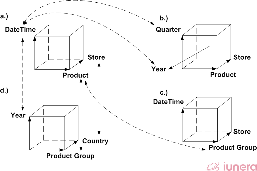
We show a subset of the original time series data that can be created with a Dice operation in a.). This subcube is the foundation to apply different operations and to do investigations with them. The other cubes b.), c.) and d.) show the outcome after different operations.

We indicate which original dimensions and attributes result in the different outcomes by linking them with dashed lines.

In the following, we discuss each resulting perspective on its own. In order to provide a better understanding, we show resulting tables in the way they are commonly used by Time Series Database or Data Warehouse exploration tools.

We also show different methods of building subtotals and totals in order to provide indications of what can be done in practice.

Nonetheless, since some operations have inverse operations that are named different we refer to both operations in the following.

For instance, when a.) is the origin as an operation to compute cube b.), it is called split. Whereby b.) to a.) is called merge.

We always mention first the “a.) to” operation name and then the inverse name in case it may exist.

With that naming guide, we first focus on the original data set in a.) and then follow up with the different operations.

We provide the point of origin in the table above, before applying advanced multi-dimensional time-series operations in a.).

In reference to our sample dataset from the beginning, we see that this dataset is a subset of the sample data that was created by a Dice operation. Therefore, only a specific product, store, date and revenues are contained in the records.

We imagine that a controller looks at the data at the beginning of his investigation. He generates charts from it and applies analytic operations. Then he decides which operations he applies for further explorations. Therefore, we imagine that he can end up with the operations that we present in the following.

Split, Merge, Pivot

The multi-dimensional Time Series Analysis Split operation is used to generate b.). Vice versa, as inversive operation Merge generates a.) from b.). The split operation increases the dimensionality of the cube.

Split can be applied to all kinds of dimensional attributes to get into specific details. Such attributes may be the store size, a store type or similar to regard every possible angle.

All together, Split and Pivot can be used to increase the dimensionality and arrange the dimensions in the desired way to reveal desired details.

Pivot is used to change the viewpoint. and to rotate rows into columns to ease computations. Therefore, often Split is applied and then the new dimensions coming out of Split are then rotated from rows to columns. Hence, we describe the outcome of a Split and Pivot operation together in the following. 

Split and Merge

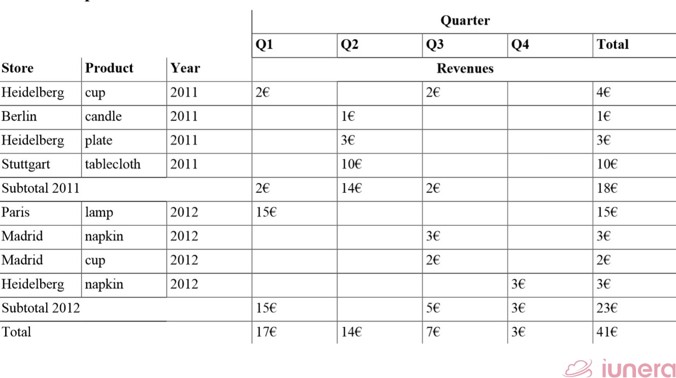
We can see that the Date is split into the year and the quarter at the same time. In contrast to the three dimensions (Store, Product, Date) in cube a.), cube b.) has now four (Year, Store, Product, Quarter).

We present the result data in the following table after we applied an additional Pivot operation for a better viewpoint. In the following, we explain the Pivot operation in more detail.

Pivot (also called Rotate)

Pivot alters the content of an axis in a spreadsheet. Therefore, it is also called rotate, because a dataset is rotated in itself.

Ultimately, the spreadsheet shows quarters arranged vertically for the years. This makes it possible to build subtotals for both; years and quarters. When we imagine a larger dataset, this gets even handier.

Currently, our time-series data has no duplicate sold products in different quarters, but we see that such issues can be handled through the total aggregation that is shown vertically. We see in the resulting totals that the quarter with the most revenues in total in Q1, followed by Q2. Furthermore, there was a rise in revenues from 18€ to 23€.

In this way, decision makers have different possibilities to Pivot the data to analyze it from different perspectives.

Roll-Up and Drill-Down

Roll-Up (c.) is decreasing the granularity of a dimension or a dimensional hierarchy. It is the “zoom-out” operator. The opposite operator is the drill down. We use this roll up operator in c.).

There, we see the product dimension generalized to the product group and all the revenues are aggregated and computed together on this level. One group may contain multiple product types, but one product has only one group. This way, the product group is a reduction of different elements.

We see the revenues for the different product groups, dates and stores. Like before, it is possible to build subtotals like for dishes or a specific store. With such subtotals, we can depict easily that dishes have been the main sold product in 2011 in the Heidelberg store.

However, in general, Roll-Ups and Drill-Down are very effective to gain an overview or an insight into a dimensional hierarchy or attributes of a dimension.

We apply a Pivot product group and exclude the date dimension to get a better overview.

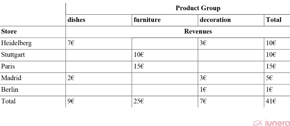
Now, we can easily depict the totals for the different stores and the various Product Groups. This reveals that furniture is responsible for the most revenues and Paris is identified to be the Store leader in revenues.

Such kind of analysis in business is used to compare the performance of stores and product groups before drilling into details.

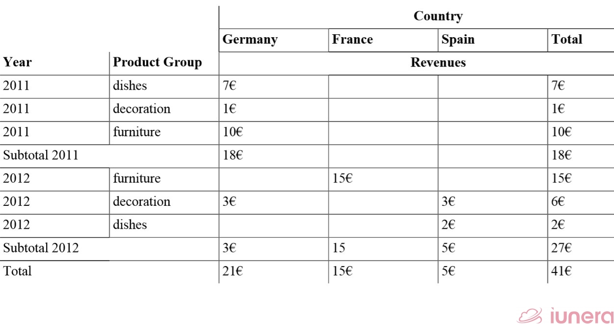
As the last operation, we show the combination of different combined Roll-Ups at the same time.

In the table, we now see the different countries in relation to Years and Product Groups. This makes it possible to depict the top Product Groups and the top-performing Countries at once.

The date has been generalized to Year, Products to the Product Group and Store to its Country. The general idea is to compare the performance of countries in different years.

In Germany, we have multiple stores and all of these stores are ragged together and their revenues are aggregated. Imagine, we have a large dataset, where all countries have multiple stores. Executives can have a look at the high-level results and work out their decisions.

Typical applications of multi-dimensional Time Series Analysis operations

Typical applications of multi-dimensional Time Series Analysis are data preparations, extractions and investigations for a certain timeframe or interval to learn more about events and data.

Slices or Dices can also support extracting data for a certain time frame to test machine learning on small examples within a certain timeframe.

Another application type is recommendation systems where different dimensionalities are used to do investigations about features.

Last but not least structured analysis, descriptive analytics and time-based aggregations are also other typical examples of where the described operations help.

Sum Up FAQ

What are the different analytical operations from Data Warehousing which can be applied for Time Series Analysis?

Slice, Dice, Pivot, Roll-Up, Drill-down, Split and Merge

What is the Slice operation for Time Series Analysis?

Slice fixes a specific dimension to a specific value. For instance, the store dimension can be fixated to a specific store.

What is the Dice Operation on Time Series Data?

The dice operation combines multiple slice operations at one time to create a subcube.

Summary and conclusion

We saw examples of the multi-dimensional Time Series Analysis operations that can be applied on Time Series Data. In special, we looked at Slice, Dice, Pivot, Roll-Up, General Roll-Up and Drill-down. Then, we referenced some exemplary applications where such operations are handy and concluded with a summary FAQ.

Now, Data Scientists and Big Data Engineers can qualify Big Data tools like Time Series Databases by their capability to execute the different operations on top of Time Series Data.

With the right tools, the data can be pre-processed better and faster before using advanced Time Series Data investigation methods. This speeds up the flexibility and improves the speed of how new insights and forecasts from Time Series Data can be revealed.

Update (29th April 2021): Check out our latest project, Fahrbar!

Related Posts

References

- V. Köppen, G. Saake, K.-U. Sattler. Data Warehouse Technologien: Technische Grundlagen. 978-3826691614. mitp Professional. 2012.
- H.-G. Kemper, W. Mehanna, C. Unger. Business Intelligence- Grundlagen und praktische Anwendungen: : Eine Einführung in die IT-basierte Managementunterstützung. 978-3834802750. Vieweg+Teubner Verlag. 2004.