
There are many types of data structures out there that are meant to store data in different ways. One of them is called a graph.
In this article, we will dive deep into what exactly is a graph and how is it used to connect and find relations between data points
Introduction to Graphs
Let us take a look at the definition of a graph from Wikipedia:
A Graph data structure consists of a finite (and possibly mutable) set of vertices or nodes or points, together with a group of unordered pairs of these vertices for an undirected graph or ordered pairs for a directed Graph. These pairs are known as edges, arcs, or lines for an undirected Graph, and as arrows, directed edges directed arcs or directed lines for a directed Graph. The vertices may be part of the Graph structure or external entities represented by integer indices or references.
Wikipedia
A Graph data structure may also associate to each edge some edge value, such as a symbolic label or a numeric attribute.
A Graph is also a non-linear data structure consisting of nodes and edges. The nodes are sometimes referred to as vertices, and the edges are lines or arcs that connect any two nodes in the graph. More formally, a Graph can be defined as below:
A Graph consists of a finite set of vertices (or nodes) and a set of Edges that connect a pair of nodes.
Graphs are mainly being used in software paradigms to obtain relations between the data points. Graphs are used to solve many real-life problems. Graphs can be used to represent a network that includes paths in a city or telephone network, or circuit network.
Types of Graphs
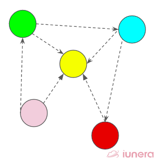
Directed Graph
In a directed graph, nodes are connected by directed edges – they only go in one direction. For example, if an edge connects node 1 and 2, but the arrow head points towards 2, we can only traverse from node 1 to node 2 – not in the opposite direction.
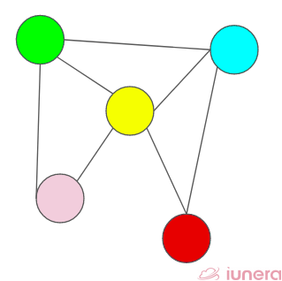
Undirected Graph
In an undirected graph, nodes are connected by edges that are all bidirectional. For example if an edge connects node 1 and 2, we can traverse from node 1 to node 2, and from node 2 to 1.
Representations of a Graph
The following two are the most commonly used representations of a graph.
Adjacency Matrix
The first approach we’ll cover uses matrices, which themselves are typically implemented as an array of arrays.
An adjacency matrix is a 2D array of size V x V where V is the number of vertices in a graph. Let the 2D array be adj[][], a slot adj[i][j] = 1 indicates that there is an edge from vertex i to vertex j. The adjacency matrix for the undirected graph is always symmetric.
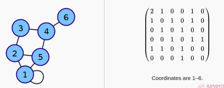
An adjacency matrix is also used to represent weighted graphs. If adj[i][j] = 1, then there is an edge from vertex i to vertex j with weight w.
Now here’s the key idea behind adjacency matrices:
Each cell in this matrix represents a connection between two nodes
Adjacency List
Now comes adjacency lists. The best way to implement this kind of graph is to think of it as a dictionary where all the nodes are keys, and the values are an array containing the nodes they are connected to.
Representing your graph using adjacency lists lets you quickly see how many nodes there are, just the number of keys in your dictionary, and how many edges there are, which is the sum of the arrays’ lengths.
In general, an adjacency list consists of an array of vertices (Array V) and an array of edges (Array E), where each element in the vertex array stores the starting index (in the edge array) of the edges outgoing from each node. The edge array stores the destination vertices of each edge.
This enables you to visit a vertex’s neighbours by reading the edge array from ArrayV[v] to ArrayV[v + 1]. One disadvantage of encoding graphs in adjacency lists is that fundamental node operations, such as determining all the connections that point to a certain node, are slightly more complex than in the adjacency matrix approach. This may scale significantly when dealing with massive amounts of data.
One of the advantages of using this method is that if the graph is sparse (there are not many edges), then adjacency lists will probably be more space-efficient than adjacency matrices.
Graph Operations
There are only 4 main graph operations that are worth mentioning.
- Check if the element is present in the graph
- Graph Traversal
- Adding elements to the graph at vertex and edges
- Finding the path from one vertex to another
Graphs Transversal Algorithms
Traversing the graph means examining all the nodes and vertices of the graph. There are two standard methods by using which we can traverse the graphs. Let’s discuss each one of them in detail.
Breadth-First Search
Breadth-first search (BFS) is a graph traversal algorithm that traverses the graph from the root node and explores all the neighbouring nodes. Then, it selects the nearest node and explores all the unexplored nodes.
‘In BFS, we traverse through one whole level of children nodes first before traverse through the grandchildren nodes. And we traverse through an entire level of grandchildren nodes before going on to traverse through other deeper nodes.’
As the name BFS suggests, you are required to traverse the graph breadthwise as follows:
- First, move horizontally and visit all the nodes of the current layer
- Move to the next layer and continue the operation
BFS uses the queue data structure to perform the transversal. The nice thing about using queues is that it keeps a reference to nodes that we want to come back to, even though we haven’t visited them yet.
Depth First Search
Depth-first search (DFS) is an algorithm for traversing or searching tree or graph data structures. The algorithm starts at the root node (selecting some arbitrary node as the root node in the case of a graph) and explores as far as possible.
The DFS algorithm can be said a recursive algorithm that uses the idea of backtracking. It involves exhaustive searches of all the nodes by going ahead, if possible, else by backtracking.
The word backtracking means when you are moving forward and there are no more nodes along the current path, you move backwards on the same path to find nodes to traverse.
All the nodes will be visited on the current path till all the unvisited nodes have been traversed after which the next path will be selected.
For a more detailed explanation of the DFS with code examples, you can visit this article.
Concepts in Graph Structures
Let us take a look at some of the popular concepts and use cases where the graph algo’s can be used in any situations.
Cycle Detection
Directed graphs are usually used in real-life applications to represent a set of dependencies. For example, a course pre-requisite in a class schedule can be represented using a directed graph. How can that be implemented? A depth-first traversal can be used to detect a cycle in a graph. DFS for a connected graph produces a tree. There is a cycle in a graph only if there is a back edge present in the graph.
Generalization in Machine Learning
Using a simple graph infrastructure, the data can be generalised in machine learning to obtain the features of the particular input subject. For example, given the node of a person with the profession, we can use graph functions and strategies to generalise the person to the profession.
Distributed Processing
Graph problems have some characteristics that make efficient parallelization not an easy task. Parallel computing, where multiple processing elements are used concurrently, offers challenges as well.
As partitioning is hard and graph computations have a varying degree of parallelism load
balancing is another challenge in the parallelization of graph processing. Active research is still being conducted on how to efficiently perform graph processing across multiple distributed systems with proper reliability and availability.
Traveling Salesman Problem (TSP)
The Traveling Salesman Problem (TSP) is a mathematical problem that involves determining the shortest yet most effective path for a person given a list of specific destinations. In the domains of computer science and operations research, it is a well-known algorithmic problem.
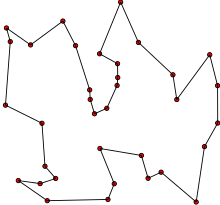
The travelling salesman problem is a graph theory optimization problem in which the nodes (cities) of a graph are connected by directed edges (routes), with each edge’s weight indicating the distance between two cities.
The objective is to find a path that visits each city just once, returns to the beginning city, and covers the shortest possible distance.
The only known generic solution algorithm that ensures the shortest path demands an exponentially increasing solution time as the size of the problem increases.
In Summary
Let us recap on what we have introduced about graphs in this article.
A Graph data structure may also associate to each edge some edge value, such as a symbolic label or a numeric attribute. There are 2 types of graph, namely directed graphs and undirected graphs. The following two are the most commonly used representations of a graph – adjacency matrices and adjacency lists.
When compared to both the implementations, one of the advantages of using this method is that if the graph is sparse (there are not many edges), then adjacency lists will probably be more space-efficient than adjacency matrices.
There are two standard methods by using which we can traverse the graphs. Breadth-first search is a graph traversal algorithm that traverses the graph from the root node and explores all the neighbouring nodes. Then, it selects the nearest node and explores all the unexplored nodes.
Depth-first search is an algorithm for traversing or searching tree or graph data structures. The algorithm starts at the root node (selecting some arbitrary node as the root node in the case of a graph) and explores as far as possible.
Extending from this context, graph database also usually constitute a central element of modern intelligent transport systems (ITS).
They play the role of an integrator through combining information retrieved from such sources as vehicles, maps, timetables, stops etc. and making it available to end-users or to store it into a data warehouse for discovering and analysing frequently used routes, bottlenecks and more.