Polyglot Knowledge RAG Ingestion Concept for Enterprise Ready AIs

Vector search is not enough for modern RAGs. It is a current AI trend to shift from pure vector search to polyglot search as even Microsoft’s NLWeb opens for elastic search for data retrival. A modular data ingestion pipeline for AI search processes, supporting diverse data types—text, images, structured content, and time series—into formats suitable for vector databases, SQL, or graph systems is the next logical step for enterprise AI. In this article, we’ll discuss a generic pipeline, optimized for AI search data preprocessing techniques beyond vector search data indexing pipelines. Inspired by modern Retrieval-Augmented Generation (RAG) frameworks, it supports scalable, polyglot data preparation and extensions for enterprise AI-driven search systems.

Understanding Retrieval-Augmented Generation (RAG)

Retrieval-Augmented Generation (RAG) integrates retrieval of relevant data with generative AI to deliver accurate, context-aware responses in search systems. RAG pipelines, used in platforms like Qdrant or Pinecone, ingest and index data (e.g., text as vector embeddings, structured data as SQL rows) for efficient retrieval. During querying, RAG employs vector similarity or SQL queries, then generates responses via LLMs like LLaMA. This pipeline’s ingestion phase ensures data is preprocessed and indexed, with extensions to handle diverse data types and indexing needs, such as Schema.org entities for structured search.

Role of Data Ingestion in AI Search

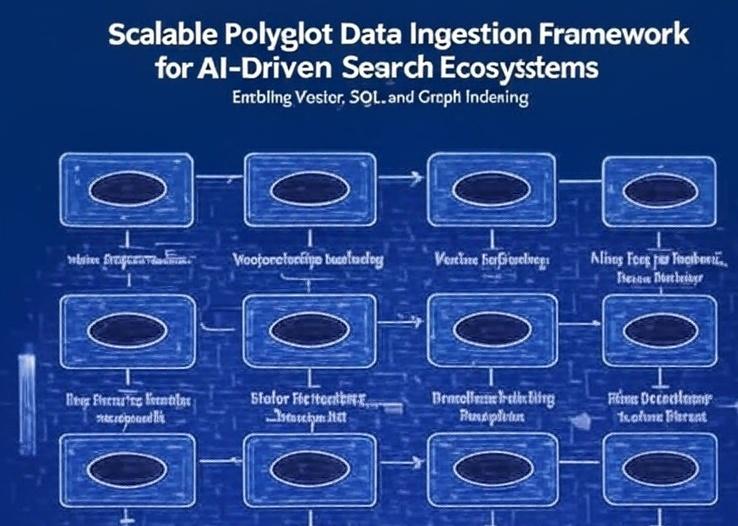
Data ingestion involves collecting, transforming, and storing data to enable querying in AI search systems. The challenge lies in managing varied data types—text for vector embeddings, images for visual embeddings, structured data for SQL, and time series for analytics databases. A modular pipeline ensures scalability by supporting tailored indexing strategies, aligning with Schema.org standards for enhanced SEO. Figure 1 illustrates this scalable data ingestion for search systems, detailing six steps with extensions for preprocessing and embedding.

Choosing the Right Database for Data Types

Selecting the appropriate database optimizes retrieval in AI search systems. Each data type requires tailored indexing for performance:

• Text Data: Stored in vector databases like Qdrant or Pinecone, using 1536-dimensional embeddings from models like text-embedding-ada-002 for semantic search. Ideal for unstructured content like articles or recipe descriptions.
• Image Data: Indexed in vector databases with visual embeddings from CLIP models, enabling similarity-based image search for product visuals or recipe photos.
• Structured JSON Data: Stored in MongoDB for flexible, schema-less storage, supporting queries on JSON fields (e.g., product attributes, recipe metadata).
• Time Series Data: Indexed in Druid or TimescaleDB for temporal analytics (e.g., user interaction logs, recipe search trends) with fast aggregation queries.
• Relational Data: Stored in graph databases like Neo4j for complex relationships (e.g., ingredient networks in recipes) or PostgreSQL for structured queries (e.g., product inventories).

This diverse indexing ensures compatibility with polyglot search, combining vector, SQL, and graph retrieval.

Limitations of Vector-Only RAG Pipelines

Many RAG systems focus solely on vector databases for text and image search, but this approach has drawbacks. Chunking, a key preprocessing step, often splits data into fixed-size segments (e.g., 512 tokens), risking loss of semantic context (e.g., splitting recipe instructions mid-step), which reduces retrieval accuracy for complex queries. Vector databases excel at similarity-based search but struggle with structured or relational data, such as product categories or ingredient relationships. Relying only on vector storage overlooks the strengths of SQL databases for precise filtering or graph databases for relational queries. A polyglot search pipeline, combining vector, SQL, and graph databases, addresses these issues by leveraging chunking for text, structured storage for JSON, and graph indexing for relations, ensuring comprehensive retrieval.

The Modular Data Ingestion Pipeline for a general purpose RAG

This 6-step pipeline transforms raw data into indexed, queryable formats, supporting AI-powered search data preparation for polyglot search. Each step includes extension points for flexibility, accommodating diverse data types (text, images, JSON, time series) and indexing methods (vector, SQL, graph). Technical details, like embedding dimensions and chunk sizes, ensure compatibility with modern RAG systems.

Step 1: Source Crawling

The pipeline begins by collecting raw data from sources like web pages, APIs, or files (e.g., JSONL, RSS feeds), using crawlers or connectors. It operates sequentially, fetching content such as recipe texts, product listings, or time series logs in JSONL format, ensuring readiness for preprocessing. 

• Process: Sequential, HTTP requests or file reads.
• Output: Raw unstructured data (e.g., JSONL, HTML content).
• Example: Crawling a recipe site for Recipe markup.

Step 2: Data Preprocessors

Data preprocessors segment raw data into manageable units, with parallel extensions for flexibility. Data enrichment extensions include:

• Visibility Specification (Roles): Adds metadata about role-based access controls (e.g., premium user access), using JSON metadata tags and associates which data should be accessible by whom.
• Chunking and Chunk Context Extension: Imagine a PDF – it is often to large to be index. Context extraction can extract the general context of the PDF and then the context is associated with each chunk when split. A chunking extension splits data into chunks (e.g., 512-token text segments). This can be done via NLTK or sentence splitting or similar means.
• Data-Type-Specific Extractions: Extracts metadata, such as image captions or processes what is to be seen on a picture via CLIP models or reasoning rules or other means.

Ultimately, this step drives AI search data preprocessing techniques, preparing data for diverse indexing and also spitting it into smaller chunks, allowing different data types to be processed differently.

• Process: Sequential, with parallel extensions (e.g., multi-threaded chunking).
• Output: Chunked data (e.g., text chunks, image metadata).
• Example: Segmenting a recipe into
  • ingredient pictures
  • result pictures
  • ingredients logical names and classifications and dimensions
  • and instructions.

Step 3: Chunked Data

This step outputs segmented data units, such as text snippets (~512 tokens), image metadata, or JSON objects, acting as a bridge to embedding. It ensures data is structured for further processing, aligning with vector search data indexing pipelines.

• Process: Sequential, prepares chunks that can sub sequentially be processed in parallel.
• Output: Independent chunked data units.
• Example: Recipe step snippets ready for embedding.

Step 4: Data Embedding

This step generates embeddings or formats data for storage, crucial for vector search data indexing pipelines. Extensions include:

• Enrichments (Filter Specification): Adds metadata filters to the data. Such filters can be based on known entities, such as Schema.org suitableForDiet: Vegetarian or recipeCuisine: Indian, enabling precise vector search queries (e.g., {"filter": {"suitableForDiet": "Vegetarian"}} in Qdrant or similar).
• Vector Embedding Generation: Creates N-dimensional embeddings for text or images using models like text-embedding-ada-002 or CLIP, per chunk.
• Embeddings for Other DBs: Formats data for other databases where other kind of relations could be inserted in addition to vector representations. E.g. prepare and extract graph relations (e.g., Neo4j node-edge structures) or SQL schemas (e.g., MongoDB JSON documents).

Outcome of this step are embeddings for different databases with optional data filters based on roles and prior filter specifications.

• Process: Sequential, with parallel extensions for different databases that produce database specific outputs.
• Output: Storage-ready data chunks (e.g., vector embeddings, SQL rows).
• Example: Embedding recipe descriptions with suitableForDiet: Vegetarian filters.

Step 5: Storage Ready Data Chunks

This output artifact contains embedded, enriched chunks formatted for specific databases (vector, SQL, graph, time series), ensuring compatibility with diverse indexing strategies. Chunks are defined in JSONL with metadata and one property can indicate which database should serve for the storage.

e.g., {database: "Qdrant","embedding": [0.0123, ...], "filter": {"suitableForDiet": "Vegetarian"}}.

Step 6: Storage in DBs

The final step indexes data in target databases, such as Qdrant for vectors, MongoDB for JSON, Druid for time series, or Neo4j for relations. Each database can have another specific extension and they can be executed in parallel. The database property in the JsonL is used to define the final storage.

This completes the modular data ingestion pipeline for AI search, enabling efficient polyglot retrieval.

• Process: Sequential, uses database-specific indexing (e.g., Qdrant’s upsert API).
• Output: Indexed data.
• Example: Indexing recipe embeddings in Qdrant, metadata in MongoDB, and trends in Druid.

Practical Implications

This pipeline enables applications like recipe search, e-commerce, or knowledge bases, supporting AI-powered search data preparation. Key considerations include:

• Clear definitions of processing points and processing chain:
  • A clear defined processing chain make sit possible to define clear plug in extension point interceptors which implement interfaces to make the process adjustable and extendable for different databases and enrichment.
  • The extension points can be defined more fine grained and be split in parallel and sequential steps to extend the processing chain even further.
  • Different default implementations make the complete chain easily configurable.
• Retrieval Differences Across Databases utilzed:
  • Vector Databases: Excel for similarity-based retrieval (e.g., Qdrant for text embeddings) using cosine similarity, ideal for unstructured text or images but limited for relationships.
  • SQL Databases: Suited for structured queries (e.g., PostgreSQL for SELECT * FROM products WHERE category='electronics'), offering precise filtering but less effective for semantic search.
  • Graph Databases: Optimal for relational data (e.g., Neo4j for recipe ingredient networks), enabling queries like “find recipes linked to Indian spices.” Best for relationships but less scalable for text search.
  • Time Series Databases: Ideal for temporal data (e.g., Druid for user interaction logs), supporting fast analytics but not semantic search.
  • Choosing the Right Database: Vector databases for semantic search, SQL for structured data, graph for relations, and time series for analytics. A polyglot search pipeline combines these for multi-faceted applications.
• Challenges: LLM costs (~$0.0001 per 1K tokens via OpenAI), data quality, and indexing complexity. However such costs can likely be reduced by using specialized low cost implementations of steps in the processing chain.
• Optimizations: With the transparent processing chain one can use local LLMs from Hugging Face or implement caching strategies or trivial keyword based embedding for efficiency.
• Future: Real-time ingestion and multi-modal support (e.g., video embeddings) align with AI research trends.

Conclusion

The modular data ingestion pipeline for AI search, visualized in Figure 1, transforms raw data into indexed formats for vector, SQL, graph, and time series databases, enabling context-aware, polyglot search applications. By supporting diverse data types, entity-based filters, and hybrid indexing, it drives scalable solutions. Developers can leverage tools like Qdrant and MongoDB to implement this vector search data indexing pipeline, enhancing AI-driven search capabilities.